
Does Visitation in Prison Reduce Recidivism
Download original document:
Document text
Document text
This text is machine-read, and may contain errors. Check the original document to verify accuracy.
Does Visitation in Prison Reduce Recidivism?
Yuki Otsu∗†
Center for Spatial Information Science,
The University of Tokyo
October 21, 2021
Abstract
Visitation in prison is associated with a low recidivism rate after release, but the
causality is not clear. This paper tries to estimate the effect of visitation experience on the recidivism outcome of state prisoners in Missouri, using an instrumental variable approach. The instrumental variable used for identification is the
distance from a prison to an address before incarceration. The results support
that visitation has a causal effect on recidivism in the short run. Further analysis
shows that employment is an important channel of the visitation effect. However,
no discernible effect on housing stability is found.
JEL classification: C26, J68, K42, R23
Keywords: recidivism, reentry, visitation, causal inference, instrumental variable
∗ Center
for Spatial Information Science, The University of Tokyo. 5-1-5 Kashiwanoha, Kashiwa,
Chiba 277-8568, Japan. Email: y.otsu@csis.u-tokyo.ac.jp
† I appreciate the staff of the Missouri Department of Correction for providing the dataset for the research project. I sincerely thank my supervisor Ian Fillmore for his support, comments, and suggestions.
I would also like to thank Marcus Berliant, George Gayle, and Robert Pollak for beneficial discussions,
comments, and advice. I also thank seminar participants at internal seminars and the Olin Brown Bag
Seminar at Washington University in St. Louis, the Happy Hour Seminar, and the UGOD seminar. The
views expressed in this paper are those of the author and do not necessarily reflect the view of the Missouri Department of Corrections. This project is approved by the IRB board at Washington University
in St. Louis: IRB ID 201904050.
1
Electronic copy available at: https://ssrn.com/abstract=3842711
1
Introduction
Since 1976, the prison population in the United States has grown rapidly such that by
2008 there were 2.3 million prisoners. Although the number of prisoners has gradually
declined since then, it has remained near peak levels over the last forty years (Bronson
and Carson, 2019), and the U.S. has one of the highest incarceration rates in the world
(Walmsley, 2015). Since most prisoners are eventually released, a high prison population implies a high rate of people with a criminal record in society. Indeed, Kaeble and
Glaze (2016) estimated that in 2015, about 7 million individuals were either in prison,
in jail, or on parole or probation, and 4.9 million people had experienced incarceration
in their past. However, it is not easy for offenders to overcome recidivism. According
to Alper et al. (2018), 68% of prisoners released in 2005 from correctional facilities in 30
states were arrested within three years of release and 83% were arrested within nine
years.
This high recidivism rate could be attributed to demographic differences. Prisoners are demographically different from those who have no criminal record: more male,
more black (Bronson and Carson, 2019), less formally educated (Motivans, 2017), and
less healthy (Maruschak et al., 2015). However, the high rate of recidivism is partially
due to the collateral consequences of incarceration. Incarceration experience and criminal records cause many problems such as discrimination in the labor market (Pager,
2003) and low employment probability (Bhuller et al., 2018; Mueller-Smith, 2015) and
is associated with unstable housing (Harding et al., 2013). Hence, removing these obstacles could be a way to reduce the recidivism rate, and it is important to know what
policies can help the reentry of prisoners into normal life.
Strong social bonds are considered as mitigating these obstacles for ex-offenders.
A social bond here means a good relationship with family, friends, and neighbors.
Family and friends can provide employment opportunities through their networks,
stable housing, and emotional support.1 Strong social bonds increase the chance of
getting this support, which is useful to overcome the obstacles. Hence, the support by
family and friends is helpful for the successful reentry of prisoners into society and
reduction of recidivism.
However, since imprisonment physically separates prisoners from family and friends,
1 Visher
and Travis (2003) surveyed literature focusing on prisoner transition back to the community.
They pointed out the importance of family ties for successful reentry, in particular, through housing
security and emotional support.
2
Electronic copy available at: https://ssrn.com/abstract=3842711
they have a hard time maintaining social ties. Correctional facilities offer several ways
for prisoners to keep in communication with those who are out of prison: letters,
phone calls, and visitation. In particular, as seen in the literature on social bonds
and recidivism, prison visitation is considered to be an important way for prisoners
to keep in communication with family and friends (Laub et al., 1998; Rocque et al.,
2013).2 The relationship between visitation and recidivism are analyzed in the literature (Visher and Travis, 2003; Brunton-Smith and McCarthy, 2017; Bales and Mears,
2008; Mears et al., 2012; Cochran and Mears, 2013; Derkzen et al., 2009; Mitchell et al.,
2016; Cochran, 2019; Lee, 2019; Cochran et al., 2020).3 The literature, for example
Visher and Travis (2003), finds that visitation experiences in prison are associated with
a low recidivism rate and claims that this effect is through social ties maintained or
improved by prison visitation. Hence, it is claimed prisons should adopt policies that
encourage visitation, relying on the idea that there is a causal effect of visitation on
the reduction of recidivism. However, most of these papers claim causality under the
assumption that there is no omitted variable bias, which is unlikely true.
Although visitation seems to be an important tool to maintain and improve social
ties and hence reduce reoffending, it is not easy to identify a causal effect of visitation
on recidivism due to endogeneity issues. Many papers have mentioned that the relationship may be causal, but most of the papers do not have a strong identification
strategy to estimate the causal effect of visitation on recidivism. We cannot conclude
that visitation has a causal effect on lower recidivism rates only from the fact that
visited prisoners have a lower recidivism rate than non-visited prisoners. It may be
strong social ties that increase prison visitation experience and reduce the recidivism
rate of ex-offenders through housing, employment, and other channels. If there is no
causal relationship, visitation experiences work as a good predictor of recidivism, but
a marginal increase in visitation may not affect the recidivism rate.
2 In
criminology, several theories are provided to explain the link between visitation and recidivism:
(1) the social bond theory, (2) the social capital theory, (3) the general strain theory, and so on. For
example, social bond theory, provided by Hirschi (1969), argues that strong social bonds with family,
friends, and community help to form norms and values that deter recidivism. The social capital theory
puts more emphasis on the support provided through strong family ties, such as money, housing, and
employment opportunities.
Although there are many theories, the focus of this paper is not to test each theory but to provide
solid evidence for those theories; these theories rely on a causal relationship existing between visitation
and recidivism, but the causality has not yet been formally investigated.
3 Since visitation can be defined in various ways, many aspects have been investigated with a recidivism outcome: relationship with visitors (Bales and Mears, 2008), frequency (Mears et al., 2012), timing
(Cochran and Mears, 2013; Bales and Mears, 2008), and length of visit (Derkzen et al., 2009). Recently,
using UK data, Brunton-Smith and McCarthy (2017) concluded visitation by parents improves family
ties and lowers reoffending of inmates.
3
Electronic copy available at: https://ssrn.com/abstract=3842711
Policymakers need to know if the relationship is actually causal, since providing
visitation opportunities requires more staff for each facility, which is costly. Despite
this, if there is any causal impact of actual visitation, it may be better to provide actual
visitation opportunities even so. Specifically, this paper identifies how much of recidivism could be reduced by one visitation and estimates the monetary costs that could
be saved by possible policies.
This paper investigates the causal effect of visitation on recidivism. To check the
causal effect and to investigate the channels of the effect, this paper uses data from
state prisoners in Missouri released between 2012 and 2015. For the identification of
the causal effect, the regression analysis is based on an instrumental variable approach.
In particular, the instrumental variable (IV) is the distance of the incarcerated prison
from the home address of the prisoner. Individuals are likely to have a social network
in their community. Hence, when prisoners are assigned to a prison that is far from
their home, they are less likely to be visited by family members or friends, simply
because the prison is far from the community; in other words, the opportunity cost of
visitation for visitors is high.
The regression results show that a negative and statistically significant effect of
visitation on recidivism: one visit per month reduces the reincarceration rate by 8
percent points. In particular, the short-run effects are robust under different samples,
control variables, and specifications.
Using the same IV approach, I also investigate the two potential channels of the
effect of visitation: employment and housing stability. According to the social capital
theory, a strong social bond is considered to provide better employment opportunities
and a labor-market opportunity is a key deterrence factor. The results indicate that
visitation increases employment probability and reduces the time to get the first job.
Similarly, housing stability is considered as another important factor since homelessness and frequent movement are associated with a higher recidivism rate. However,
the estimation results do not show any effect on housing stability. Hence, the employment channel is more important than the housing channel to explain the visitation
effect. Finally, as a result of a back-of-the-envelope calculation, the state government
can save the expenditure per inmate by 813 dollars at the median if every prisoner
were assigned to the closest prison.
This paper advances the literature in two ways. First, this paper provides empirical support for the literature about visitation and recidivism. An official report by the
4
Electronic copy available at: https://ssrn.com/abstract=3842711
Minnesota Department of Corrections (Minnesota Department of Corrections, 2011)
concludes one visitation reduces the risk of recidivism by 13% for felony convictions
and 25% for technical violation revocation. However, the report is based on a simple
Cox hazard model and hence, as mentioned in the report, the estimator shows a correlation rather than causality. Most other papers show a correlation between visitation
and recidivism. Cochran et al. (2020) and Lee (2019) are two recent papers that use a
similar IV approach to check the causal effect of visitation on recidivism using state
prisoners in Florida and Iowa, respectively.4 They cast doubt on the causality because
they did not find a causal effect on recidivism. However, they measured a recidivism
outcome only at three years from release. Using administrative data in Missouri, this
paper supports that visitation has a causal effect and helps successful reentry. The
results suggest that the key differences are the time when the recidivism outcome is
measured.
Second, this paper contributes to the literature on the channels of the visitation
effect: specifically employment and housing. The literature shows that better employment opportunity decreases recidivism rate (Yang, 2017; Schnepel, 2018). Higher
wages (Yang, 2017) and more vacancies (Schnepel, 2018) in local labor markets reduce
the recidivism rate. Unstable housing is associated with higher recidivism outcomes
(Geller and Curtis, 2011). However, the visitation literature mainly focuses its effect
on recidivism, but the channels of the effect are not well-investigated (Cochran, 2019).
This paper fills this gap by investigating the effect on employment and housing outcomes. The results provide evidence that visitation improves employment outcomes
but no evidence of improvement in housing stability.
2
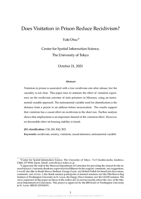
Theory
Figure 1 summarizes the conceptual framework of why visitation improves the recidivism outcome. Prisoners are sent to a prison with an initial level of social ties.
Social ties in this context mean connections with families, friends, and communities.
During the imprisonment, the level changes through visitation experiences. The visitation experiences are affected by the initial level of social ties as well as the distance
4 Cochran
et al. (2020) used the distance to the first prison assigned to as an IV to predict visitation
experiences, and Lee (2019) checked several measures of distance from the prison. In both papers, the
result of the instrumental variable regression shows an insignificant effect of visitation on recidivism
within three years, and hence they are skeptical of any causality.
5
Electronic copy available at: https://ssrn.com/abstract=3842711
Incarceration
Release
Employment
Distance
Initial Social Ties
Visitation
Crime
Social Ties
Housing
Figure 1: Conceptual framework
to prisoners’ homes from the prison. The initial level of social ties and visitation experiences determine the social ties at release, and the social ties affect post-release behavior. Social ties affect the recidivism outcome both directly and indirectly through
employment and housing situation.
Strong social ties increase opportunities to get job offers after release. Having
more and reliable connections with others increases job opportunities through their
networks. Employment has been considered as a desistance tool. Chalfin and McCrary (2017) surveyed the literature on crime and employment and concluded that
employment is a tool to reduce crime. One reason is that legal income becomes the
opportunity cost of crime (Becker, 1968). Another reason is time allocation: engaging
in a legal job as an occupation reduces the time spent on illegal activities. This relationship holds for ex-prisoners. Schnepel (2018) found that released prisoners are less
likely to recidivate when local labor markets are strong: that is, more vacancies. Yang
(2017) also reached a similar conclusion using different data.
Social ties are also considered an essential factor for the stability of the housing situation (Visher and Travis, 2003). Geller and Curtis (2011) summarized why housing
security is important for ex-prisoners.5 Stable housing helps ex-prisoners to become
employed, to access social services such as healthcare, and to keep in contact with parole officers. Moreover, loitering or homelessness increases contact with police officers,
which increases the probability of reincarceration.6
5 Frequent
movement or homelessness is considered as a bad signal for recidivism. Harding et al.
(2013) found a low rate of homelessness but high residential mobility among former prisoners, partially
due to discrimination in the housing market.
6 However, movement to a new location may reduce recidivism. Moving to a place far from home
makes people less likely to recidivate, since the move makes it difficult to keep the former criminal
6
Electronic copy available at: https://ssrn.com/abstract=3842711
The relationship between the housing situation and crime relates to housing policies. Housing support could be helpful to get a job, and employment eventually reduces crime through the opportunity cost. For example, low-income housing developments reduce violent crimes in poor neighborhoods (Freedman and Owens, 2011),
and an emergency financial assistance for those who cannot pay the rent for the current month reduces crime (Palmer et al., 2019).7
There are other channels through which social bonds affect recidivism. A line of
literature in criminology emphasizes the importance of support from others. In particular, family support is considered an important factor in reducing recidivism. Using survey data, Naser and La Vigne (2006) found that prisoners rely on family for
both material and emotional support. For example, material support, such as social
welfare, health care, and transportation, could affect recidivism. Another important
channel is the emotional channel, which could directly affect criminal behavior. For
example, peer effects of criminal behavior have been analyzed in network literature
in economics. Depending on the peers, the peer effect could improve or worsen postrelease behavior (Corno, 2017). Moreover, social ties construct social norms that emotionally deter criminal behavior as described by the general strain theory.
Even though I have explained these channels separately, they are interrelated. Stable housing helps to have a job, and a job helps to have stable housing, since it makes
the rent payment more likely. Family support helps stable housing, since ex-prisoners
can live together with their family or receive help to rent an apartment. Also, family
and friends’ support can introduce job opportunities through their existing networks.
Hence, it is important to note that this paper aims to estimate the overall effect of
visitation on a recidivism outcome.
In summary, visitation improves social ties and improved social ties change postrelease criminal behavior through employment, housing stability, and other channels.
network around the community (Kirk, 2009).
7 Since the financial assistance could be used for another purpose, the result may represent an income
effect.
7
Electronic copy available at: https://ssrn.com/abstract=3842711
3
Data
3.1
Summary Statistics
The data used for this paper are administrative data obtained from the Missouri Department of Corrections. The sample for the analysis consists of parolees and probationers in Missouri released between 2012 and 2015. Although the analysis in this paper is limited to parolees and probationers, they account for more than 90 % of released
prisoners. Each observation is based on a cycle defined by the admission date and the
release date. For each observation, the data contain residential and employment information during supervision and recidivism outcomes until 2019 August; hence the
data contain complete information on recidivism for at least three years. It is important to note that the recidivism results are based on records in Missouri. Therefore,
incarceration in other states is not included in the data.
A recidivism measure in the paper is defined as a return to incarceration. By definition, it contains a supervision condition violation.
Visitation could be measured in several ways. In particular, this paper uses the following two measures: visit dummy and visit frequency over the entire sentence period.
Visit dummy is a binary measure of visitation experience that takes one if someone
(family, friends, etc.) visits the offender while incarcerated, and zero otherwise. Visit
frequency is the number of total visitations over incarcerated months.
Among all released prisoners on parole or probation, the sample used for the analysis satisfies the following conditions: (1) male, (2) at working age, (3) living only in
Missouri during supervision, and (4) serving an original sentence. Given that most
prisoners are male, it is reasonable to focus on the male sample for the analysis. Moreover, gender might have correlated with the distance between home and prisons, since
most of the prisons are for males. The sample is limited to those of working age (20–65)
at release to focus on the employment channel. An out-of-state sample is excluded to
avoid a selection problem.8 Lastly, this paper focuses on an initial cycle for a sentence:
in other words, not a cycle for parole revocation. Some observations are dropped during the data cleaning process, such as missing values. Finally, 33,971 observations are
used for the analysis. Note that since each observation consists of one cycle from incarceration to release, one person could have multiple observations when the person is
8 Out-of-state sample has a lower recidivism rate because of the following two reasons. One is that return to prisons in other states is not recorded in the Missouri database. Another reason is that prisoners
have to behave well to get approval for the interstate supervision.
8
Electronic copy available at: https://ssrn.com/abstract=3842711
51.3
50.0
48.2
43.7
40.0
41.1
30.0
26.0
22.7
20.0
11.5
10.0
8.6
Not Visited
Visited
0.0
6 month
1 year
2 year
Time from Release
3 year
Notes: The lines show the recidivism rate of male prisoners over time
with the confidence interval (CI). The CI is at 95% level.
Figure 2: Reincarceration rate over time
released, incarcerated, and released again between January 2012 and December 2015.
Basic demographics are summarized in Table 1. The mean age at release is 35.1,
and 70% of observations are below the age of 40. Non-Hispanic whites and blacks
account for almost all observations and other ethnic groups such as Hispanics, Asians,
and Native Americans are rare.
Table 2 compares demographics by visitation experience. The visited group is prisoners who experienced visitations at least once while in prison. The visited group has
similar characteristics with the non-visited group, but the sentence length is longer.
This is likely because the more time they spend in prison, the more chances they will
be visited.
3.2
Post Release Outcomes
Figure 2 summarizes the recidivism rate for up to three years since release. At six
months from release, 8.6% of the visited group returns, while 11.5% of the non-visited
group returns. The difference remains stable over time. At three years since release,
48.2% of visited prisoners return, while 51.3% of non-visited prisoners return. Overall, as seen on the graph, visitation experience is associated with a relatively lower
recidivism rate by about 3% points.
9
Electronic copy available at: https://ssrn.com/abstract=3842711
Table 1: Summary statistics
N=33,971
Mean
Distance (mile)
114.31
Age at Release
35.09
Race/Ethnicity
White (Non-Hispanic)
0.66
Black (Non-Hispanic)
0.24
Other Race
0.10
Sentence Length
5.58
Parole
0.70
Primary Crime Type
Property
0.29
Violent
0.13
Drug
0.28
Other Crime
0.30
Felony Class
A (10-30 year)
0.02
B (5-15 year)
0.17
C (3-10 year)
0.65
D (-7 year)
0.15
Custody Level
Low
0.39
Medium
0.39
High
0.22
Reincarceration
within 6 month
0.10
within 1 year
0.24
within 2 year
0.42
within 3 year
0.50
Supervision Completion
0.35
Employment
ever since release
0.47
at 3 month from release
0.23
at 6 month from release
0.29
Fulltime (ever since release) 0.39
Movement (Dummy)
0.55
Movement (Freq. per month)
0.07
S.D. Min
68.79 .706
10.18 20
Max
385
64.9
0.47
0.43
0.29
3.06
0.46
0
0
0
0
0
1
1
1
50
1
0.46
0.34
0.45
0.46
0
0
0
0
1
1
1
1
0.15
0.38
0.48
0.36
0
0
0
0
1
1
1
1
0.49
0.49
0.41
0
0
0
1
1
1
0.30
0.43
0.49
0.50
0.48
0
0
0
0
0
1
1
1
1
1
0.50
0.42
0.45
0.49
0.50
0.16
0
0
0
0
0
0
1
1
1
1
1
15
Notes: Supervision completion is defined as a share of “Discharge” over sum of “Abscond”, “Revoke”,
and “Discharge”. The other outcome “Death”, which account for 6.7% of overall sample, is not included.
10
Electronic copy available at: https://ssrn.com/abstract=3842711
Table 2: Mean by visitation experience
Distance (mile)
Age at Release
Race/Ethnicity
White (Non-Hispanic)
Black (Non-Hispanic)
Other Race
Sentence Length
Parole
Primary Crime Type
Property
Violent
Drug
Other Crime
Felony Class
A (10-30 year)
B (5-15 year)
C (3-10 year)
D (-7 year)
Custody Level
Low
Medium
High
Reincarceration
within 6 month
within 1 year
within 2 year
within 3 year
Supervision Completion
Employment
ever since release
at 3 month from release
at 6 month from release
Fulltime (ever since release)
Movement (Dummy)
Movement (Freq. per month)
Not Visited
Visited
N=17,784
N=16,187
Mean
S.D.
Mean
125.7
70.9
101.8
35.7
10.6
34.5
S.D.
64.1
9.71
0.64
0.26
0.098
5.16
0.63
0.48
0.44
0.30
2.81
0.48
0.68
0.23
0.093
6.04
0.77
0.47
0.42
0.29
3.26
0.42
0.29
0.10
0.30
0.31
0.45
0.30
0.46
0.46
0.30
0.16
0.25
0.29
0.46
0.37
0.44
0.45
0.012
0.14
0.68
0.17
0.11
0.35
0.47
0.37
0.038
0.21
0.62
0.13
0.19
0.41
0.49
0.34
0.46
0.30
0.24
0.50
0.46
0.43
0.32
0.49
0.19
0.47
0.50
0.39
0.11
0.26
0.44
0.51
0.32
0.32
0.44
0.50
0.50
0.47
0.086
0.23
0.41
0.48
0.39
0.28
0.42
0.49
0.50
0.49
0.40
0.19
0.24
0.32
0.54
0.079
0.49
0.39
0.43
0.47
0.50
0.19
0.54
0.28
0.33
0.47
0.56
0.070
0.50
0.45
0.47
0.50
0.50
0.12
11
Electronic copy available at: https://ssrn.com/abstract=3842711
50
15000
40
12000
20
30
% Ever Visited
Total Counts
6000
9000
10
3000
Enter
.25
Counts
CDF
.5
.75
Visitation Timing over Cycle
0
0
...
Release
Figure 3: Visitation timing
As seen in Table 2, the visited group has a higher supervision completion rate and
are more likely to have employment since release. More than half of the released prisoners experienced at least one movement (change of the address) during supervision.
3.3
Visitation
Figure 3 shows the visitation timing over the sentence period. The fraction of people
who have ever been visited increases over time. However, the total counts of visits
peak in the middle and then decrease as the release date approaches.
Figure 4 summarizes the visitation experience by the relationship between prisoners and visitors. The fractions indicate those who have been visited by the visitor type
at least once during incarceration. The category Others contains persons such as attorneys and clergy. The number does not sum up to one, since visitation by multiple
types of people is possible. The figure indicates that 48% of the sample has an experience of visitation by someone at least once. 38.7% of the sample is visited by relatives
and 25.4% is visited by friends. Visitation by relatives is more common than friends
or others. Among relatives, mothers are the most common as a single category, and
1 in 5 observations experienced a mother’s visitation. Only 6.2% of prisoners experience visitation by a spouse, but since 20% of the sample reported being married at the
initial classification, 1 in 4 married observations experienced spousal visitation.
12
Electronic copy available at: https://ssrn.com/abstract=3842711
50
Ever Visited by the group (%)
10
20
30
40
47.6
38.7
26.3
25.4
23.1
15.0
10.1
9.2
6.2
O
th
er
s
s
nd
ie
n
re
ld
hi
Fr
er
O
th
nt
ca
Si
gn
ifi
C
e
us
er
Sp
o
th
Fa
ot
he
r
ts
M
en
Pa
r
R
el
at
iv
An
y
es
0
2.3
Notes: This graph shows the fraction of prisoners visited by the category during incarceration. Relatives
and parents are aggregated categories. Relatives include parents, spouses, children, and other relatives,
and parents contain mother and father. The sum of the fractions of mother and father is not equal to the
fraction of parents, since some prisoners experience visitation by both.
Figure 4: Visitation by relationship
3.4
Prison environment in Missouri
3.4.1
Prison assignment process
Before the regression analysis, this section summarizes the prison assignment process
in Missouri. Once the sentence is determined, prisoners are sent to one of the Diagnostic Intake Centers for initial classification. Based on gender, special needs, and
the custody level determined by the classification, an offender is assigned to an initial prison.9 During incarceration, the custody level is updated periodically. Typically,
the first reclassification of the custody level happens about six months from the initial
assessment, and after that, reclassification is completed every 12 months.
Each prisoner is assigned one of three levels of custody: minimum, medium, and
maximum. In principle, the custody level is determined by the maximum of two
scores: institutional score (I score) and public risk score (P score).10 The I score is
calculated by certain variables: age, most serious offense, mental health, education,
9 See
Missouri Department of Corrections (2013) for a complete description of the classification process.
10 This rule may not be so strict in practice because some are assigned a lower custody level than their
P score. However, the number of such observations is only 552, which accounts for only about 1.6% of
the total sample, so the problem is not severe.
13
Electronic copy available at: https://ssrn.com/abstract=3842711
•
0
0
-
M
in
im
u
m
M
ed
iu
m
M
ax
im
u
m
1
0
1-1
,0
0
0
1
,0
0
0-3
0
,0
0
0
3
0
,0
0
0-1
7
9
,5
3
3
K
a
n
sa
sC
ity
S
t.L
o
u
is
I
0
I
2
5
5
0
1
0
0M
iles
Notes: There are 19 correctional facilities for male prisoners in Missouri and each facility has its security
levels. Prisons with small, medium, and large circles indicate minimum, medium, maximum security
levels, respectively. There are only 16 points in the map, since 3 facilities are adjacent to other facilities.
The gradation of red color is based on total crime counts over 4 years (2012–2015).
Figure 5: Missouri state prisons for male
vocational skill, and conduct violations (for both the initial and reassessment), employment status, marital status, revocations, incarceration history (only for an initial
assignment), and program failure (only for reassessment). The P score is based on the
seriousness of the pending charge, remaining sentence, program completion, conduct
violation, and prior escape. As of June 30, 2015, 36.4% of male prisoners are assigned
the lowest risk and 35.9% and 27.7% are assigned medium and maximum level, respectively (Nixon and Lombardi, 2015).
3.4.2
Prison locations
In Missouri, there were 22 correctional facilities as of the end of 2015. Since two prisons among them were for females11 and another one had switched from a community
release center to a prison in late 2015, the analysis focuses on 19 correctional facili11 There
are only two facilities for female prisoners, which are located in the north of Missouri
(Audrain County and Livingston County). Both can accommodate prisoners of any custody level. Since
the possible variation of distance is limited, the main section of this paper focuses on male prisoners.
The analysis of female prisoners is in Section 5.2.1.
14
Electronic copy available at: https://ssrn.com/abstract=3842711
ties. Figure 5 shows the locations of the facilities. Prisons are roughly concentrated
along a line from northwest to southeast, and the southwest region has a few prisons
only. Missouri has two major cities: St. Louis and Kansas City. There are multiple maximum-security facilities near St. Louis but not many near Kansas City. Each
facility has its security level: Minimum, Medium, and Maximum. Some facilities accommodate offenders of multiple security levels. Six prisons have all security levels
and two facilities that have medium and maximum levels locate next to other levels of
prisons.12
Figure 5 also shows the number of reported crimes by county from 2012 to 2015.
The number is high in large cities such as St. Louis City and County, Kansas City, and
Columbia. Prison locations are not concentrated in high crime rate counties, however.
3.4.3
Visitation process
In order to receive visitation, Missouri prisoners have to submit a list of potential visitors, and the list can have at most 20 persons. Prisoners can update the list at most
twice a year.13 Generally, prisons accept visitors from 9:30 to 13:30 and 14:30 to 18:30
on Friday, Saturday, and Sunday, although there are slight differences across facilities.
4
Approach
4.1
Regression model
The regression is based on the following specification:
yitpc = α + β visit visitit + β X Xit + ηt + η p + ∑ ηcj 1(custody = j) + eitpc .
(1)
j∈ J
An outcome variable yitpc is a binary indicator of outcome after the release of a
person i who is from a county c, incarcerated in a prison p,14 and released at time
12 Most
prisons were open during the entire sample period (2003–2015), except ERDCC and JCCC,
which opened in 2003 and 2004, respectively. Some inmates were assigned to facilities other than the 19
discussed above. For example, two prisons existed for a short time in the sample period: the Missouri
State Penitentiary (MSP), which closed in 2004, and the Kansas City Reentry Center (KCRC), which
switched from the Kansas City Community Release Center in 2015. Moreover, inmates could also be
assigned to community release centers during incarceration. However, this paper does not use these
cycles for the analysis because they are rare.
13 For more information about the regulations, see Precy and Greitens (2018).
14 Offenders can be assigned to multiple prisons over one sentence. p is defined as the initial prison
where a prisoner is assigned after the initial risk assessment.
15
Electronic copy available at: https://ssrn.com/abstract=3842711
t. Visitit is a measure of visitation experience while imprisoned. Xit is a vector of
control variables at the time of release.15 ηt and ηcj are time and county fixed effects,
respectively. The county fixed effects ηcj are defined separately for each custody level
j ∈ J = { Min, Med, Max }. The prison fixed effects η p capture the prison-specific
factor such as job training and an education program. Standard errors are clustered at
county level. The regression coefficient of interest is β visit and the coefficient measures
the effect of visitation experience on recidivism.
The regression is based on a linear probability model (LPM). Since visitations are
count data, Poisson and negative binomial models are standard, especially, in the literature in criminology. However, this paper uses LPM rather than nonlinear models
because LPM is superior when interpreting the marginal effect. Since the objective is
to check the effect of an additional visit on recidivism, and this paper uses different
measures of visitation including continuous measures, LPM is better than other nonlinear models such as Logit and Probit. The coefficient under the LPM captures the
local average treatment effect (LATE).
As claimed in the literature, the expected sign of β visit is negative. However, the
OLS regression may suffer an omitted variable bias. Possibly the bias stems from
the strength of social bonds. When strong social bonds increase visitation as well
as decrease reoffending behavior, the OLS estimator could overestimate the negative
impact of visitation in magnitude. Hence, this paper uses an instrumental variable
approach to check a causal effect.
4.2
Explanatory variables
Control variables are demographics (age at release, race/ethnicity, and number of dependents), crime information (felony class, the primary type of crime, sentence length)
and the initial custody level.16 The complete list and detailed information of control
variables are in the Appendix. Three fixed effects are included in the model: prison,
time, and county by custody level fixed effects.17 Prison fixed effects capture the dif15 The
list and details of the control variables are in the appendix A.
(2019) used LSI-R score to control existing family factors. However, MDOC uses the Salient
Factor Score instead of LSI-R to calculate the risk of recidivism. Moreover, incarceration history is not
available. The Salient Factor (SF) score is an index based on some demographic variables, criminal
history, and behavior while incarcerated. Since visitation could affect the SF score through misconduct,
the score is not included as a control variable in the main regression. The regression results with the SF
score are in Section 5.2.1.
17 In other words, estimation uses the variation of recidivism rates net of mean differences across
prisons, times, and county-custody pairs.
16 Lee
16
Electronic copy available at: https://ssrn.com/abstract=3842711
ference across prisons such as a rehabilitation program offered in a specific prison.
Time fixed effects are to capture the effect by economic conditions, since, as Schnepel
(2018) and Yang (2017) pointed out, better economic conditions at the time of release
provide better employment opportunities and better opportunities in legal sectors of
the economy eventually decrease criminal behavior. County by custody level fixed
effects capture time-invariant county characteristics. Hence, the county by custody
level fixed effects control a consistently higher crime rate in big cities such as St. Louis
and Kansas City. Most importantly, the fundamental distance to correctional facilities
is captured by the county by custody level fixed effects.18 As Bedard and Helland
(2004) found, criminals may commit a crime taking less visitation into account when
their home is far from any prison. By including the county by custody level fixed effects, the distance term in the first stage regression captures the unexpected variation
of distance. It is worth noting that the county by custody level fixed effects are defined
for each custody level (Min, Med, Max) to capture the unexpected distance, which is
discussed more in detail in the next section.
4.3
Instrumental variable
The identification of the causal effect relies on an instrumental variable approach. An
instrumental variable for visitation is a distance from prisoners’ home to the prison
they were in.19 The reason why distance could be correlated with the visitation experience is that people have social ties locally based on the residential location, and
families and friends likely live in the neighborhood. Hence, when prisoners are assigned to a prison that is far from their home, they are less likely to be visited by their
family members or friends. The literature found a correlation between more distant
prisons and less visitation (Mears et al., 2012; Cochran et al., 2020).
Since the data do not have the exact address of each prisoner before incarceration,
the county of conviction is used as a proxy of an initial address before incarceration
following Schnepel (2018) and Cochran et al. (2020).20 The measure of distance used
18 Mcclellan
et al. (1994) used a distance to the hospital as the instrumental variable to check the
effect of intensive treatment on mortality. They also conditioned on the distance to the closest hospital
to avoid potential confounders such as urban-rural differences. Cochran et al. (2020) and Lee (2019)
controlled the average distance by county fixed effects.
19 Physical distance has been used as an instrumental variable in other papers (Mcclellan et al., 1994;
Baiocchi et al., 2010; Cochran et al., 2020; Lee, 2019).
20 County of conviction is determined by the place of the offense. This may not be a good proxy of
residential address when people commit crimes at a place far from their homes. However, crime is a
local phenomenon; Bernasco (2010) showed that 75% of burglaries are committed within five kilometers
17
Electronic copy available at: https://ssrn.com/abstract=3842711
.008
.006
Density
.004
-
-
-
.002
-
-
-
0
n_ 0
100
200
Distance (mile)
n-...... n
300
400
Notes: The vertical line is at the mean. Home address is based on counties of conviction.
Figure 6: Distance from home
in the analysis is the linear distance from the geometric center of counties to prisons.21
Since there are 115 county-equivalent areas22 and 19 state correctional facilities for
male prisoners in Missouri, there are 2185 pairs of a county and a prison.
The prison used to compute the distance is set to the first prison assigned after the
initial risk assessment. Sometimes prisoners experience a transfer from the first facility
to another correctional facility. In the data, 38% of the observations experience more
than one transfer. However, this paper does not use the distance to the second or later
prisons since the transfer decisions take into consideration some factors potentially
problematic to the validity of the instrumental variable (Precy and Greitens, 2018).
For example, to keep good institutional conduct is one of the factors but this may
generate a correlation between the distance and family ties, since the distance may
affect institutional misconduct through visitation as showed in Mears et al. (2012).
Another problematic factor is the request from prisoners to be assigned to a facility
close to their families. The request could also generate a correlation between distance
and family ties. Hence, this paper uses the distance to the first facility after the initial
risk assessment. The distribution of the distance is in Figure 6.
and about 90% is committed within ten kilometers from home in the Hague, Netherlands.
21 Road distance could be the best proxy. However, since location data is county level and travel time
within a county could be large, this paper does not use the travel time.
22 Missouri state has 114 counties and one independent city (St. Louis City).
18
Electronic copy available at: https://ssrn.com/abstract=3842711
4.3.1
Identification assumptions
This paper uses a distance from prisoners’ homes to their prison as an instrument.
With the instrumental variable approach and some conditions, the estimated coefficient β visit in the equation (1) is the local average treatment effect (LATE) of visitation
(Imbens and Angrist, 1994): the average treatment effect among the compliers. In this
context, a complier is someone who can experience visitation if assigned to a nearby
prison but not if assigned to a distant prison. For the estimation of the LATE, this
paper assumes the following conditions: (1) the distance correlates with the visitation variable (relevance), (2) the distance is correlated with an outcome variable only
through the visitation variable (exclusion restriction), and (3) visitation decreases with
distance (monotonicity).
Relevance and monotonicity are confirmed in Figure 7. Figure 7 plots visitation
experience and distance. Both figures show that the longer the distance, the lower
the fraction of prisoners that experiences visitation. The extensive margins of visitation seem to have a linear relationship. However, the means of the intensive margins
drop more at a lower distance. The non-linear relationship for intensive margins was
also found in Lee (2019). Hence, the figures support the relevance and monotonicity
conditions of the instrumental variable.
The exclusion restriction is related to the assignment process. The assignment is
influenced by two factors: the custody level and county of origin. As I discussed
in Section 3.4.1, the custody level is an important factor in the assignment process
because it determines a possible set of prisons a prisoner can be assigned.
Moreover, the assigned prison tends to be closer to the county of origin. Figure
8 shows the origin of prisoners at each correctional facility. The figure indicates that
each facility accommodated more prisoners from the neighborhoods.
However, the assignment is not deterministic: people from the same county and
custody level are assigned to different facilities. The source of variation is capacity
constraints. Since the sample period is during the period of mass incarceration, the
correctional facilities in Missouri have chronically faced a shortage of available beds
for prisoners, which generates randomness in the assignment process. Hence, conditional on the two key factors, the custody level and county of conviction, the assignment can be regarded as random, and the identification of visitation effects relies on
the unexpected variation of the distance. To control for the custody level and county
19
Electronic copy available at: https://ssrn.com/abstract=3842711
.8
0
.2
Visitation Experience
.4
.6
•
••••
• • ••
•
•
• •• • •• ••• •• •• •• ••
• • • • ••
• •• •••
•
• •
• • •• •
0
50
100
150
Distance (mile)
200
250
Visitation Frequency per month
.01
.02
.03
.04
.05
(a) Extensive margin
• •
• •• ••• •••••••••••••
• ••
••••
• •• •••• •
•• • • • •
0
•• •
• ••
0
50
100
150
Distance (mile)
200
250
(b) Intensive margin
Notes: The point at the longest distance in the figure is the mean of all observations that exceed 250
miles.
Figure 7: Visitation experience by distance
20
Electronic copy available at: https://ssrn.com/abstract=3842711
ACC
CTCC
ERDCC
FCC
JCCC
MCC
MECC
MIC
NECC
occ
PCC
sccc
SECC
WRDCC
(4 .00,ll.OO)
(2.00,4 .00)
(1.33,2.00)
(0.00,1.33)
(-0.25,0.00)
(-0.50,-0.25)
(-0.75,-0.50)
[· l.00,·0.75)
Notes: A circle in each graph represents the location of the facility. The color of each county is based
on the share of prisoners from the county relative to the state average. A red (blue) color in a graph
means the share of prisoners from the county is higher (lower) than the share of prisoners in the entire
sample.
Figure 8: Origin of prisoners by prison compared to the statewide mean
21
Electronic copy available at: https://ssrn.com/abstract=3842711
of origin, the explanatory variables in the regression include the county fixed effects
for each custody level.
Table 3 confirms the correlation of distance with observable variables by the OLS
regression. The result shows that distance correlates with some variables, but not in
an unexpected way. The positive correlations with sentence length and the violent
crime indicator are because of the severity of the crime. Longer sentence length and
violent crime tend to assign a higher custody level. Since high-security level prisons
are relatively rare, a higher custody level correlates with longer distance. The negative correlation with drug crime was also confirmed by Lee (2019), although it was
insignificant in Lee (2019). Lastly, non-Hispanic blacks tend to have longer distance
than non-Hispanic white, since blacks concentrate in particular counties.23 In the sample, 59% of non-Hispanic blacks come from the top three counties (St. Louis City, St.
Louis County, Jackson County), while only 15% of non-Hispanic whites are from the
top three counties (St. Louis County, St. Charles County, Greene County).
In summary, the key factors in deciding the assignment are the custody level and
the origin of prisoners. Conditional on the same custody level and the same sentencing
county, the assignment could be considered as random.
5
Main results
5.1
First stage
The first stage regression results confirm the distance has a strong correlation with visitation in Table 4. For the estimation shown in Table 4, all control variables and fixed
effects are used as explanatory variables. The estimated coefficients show that an increase in the distance by 100 miles reduces the chance of visitation by 7.4 percentage
points and the monthly frequency by 17.8 percentage points. The large first-stage F
statistics indicate that the distance is a strong instrumental variable for the two measures of visitation (Stock and Yogo, 2005). Hence, the first-stage results support that
the distance is a valid instrumental variable in terms of the strength of the correlation.
23 Section
5.2.3 checks the racial heterogeneity of the effect.
22
Electronic copy available at: https://ssrn.com/abstract=3842711
Table 3: Correlation with distance
Distance
Age at Release
Sentence Length
Non-Hispanic Black
Other Race
Dependents
Violent Crime
Drug Crime
Other Crime
Felony Class B
Felony Class C
Felony Class D
Custody Level (Medium)
Custody Level (High)
Controls
Prison FE
County by custody FE
Time FE
Observations
(1)
All
(2)
Not Visited
(3)
Visited
-0.0520*
(0.0289)
0.667***
(0.117)
1.555*
(0.798)
-1.537
(0.994)
-0.280*
(0.158)
3.607***
(0.938)
-2.301***
(0.753)
0.173
(0.805)
-2.626
(1.992)
-3.383*
(2.019)
-4.723**
(2.229)
-19.39**
(9.079)
15.33
(10.08)
-0.0493
(0.0371)
0.804***
(0.164)
-1.699
(1.053)
-1.185
(1.316)
-0.286
(0.216)
4.886***
(1.366)
-2.814***
(0.984)
0.0923
(1.070)
-3.778
(3.560)
-5.541
(3.567)
-7.866**
(3.781)
-15.95
(14.34)
12.71
(12.30)
-0.191***
(0.0452)
0.691***
(0.168)
3.330***
(1.190)
-3.000**
(1.468)
0.0272
(0.227)
3.313***
(1.274)
-2.263**
(1.132)
0.310
(1.185)
-1.308
(2.436)
-2.103
(2.498)
-1.890
(2.875)
-19.57
(12.24)
20.39
(16.50)
Y
Y
Y
Y
33,971
Y
Y
Y
Y
17,784
Y
Y
Y
Y
16,187
Standard errors are clustered at county level. *** p<0.01, ** p<0.05, * p<0.1.
23
Electronic copy available at: https://ssrn.com/abstract=3842711
Table 4: First stage
(1)
Dummy
(2)
Frequency
-0.0740***
(0.00685)
-0.178***
(0.0172)
Y
Y
Y
Y
33,971
116.9
Y
Y
Y
Y
33,971
107.6
Visitation
Distance (100 miles)
Controls
Prison FE
County by custody FE
Time FE
Observations
First-Stage F Statistic
5.2
The effect on recidivism
The regression results are summarized in Table 5 and 6. The first column shows the
OLS results and the second column shows the IV regression results. Each row shows
a result of recidivism outcomes at four points (6, 12, 24, and 36 months from release).
Visitation is measured by a dummy variable in Table 5, and by frequency per month
in Table 6.
In the OLS, the estimated coefficients show a negative correlation between visitation and recidivism. Visitation experience is associated with 3–6% point lower recidivism rates, and one visitation per month is associated with a 1–3% point lower
recidivism rates.
The IV results have larger negative effects than the OLS results, which is also confirmed by Cochran et al. (2020). Based on the estimators in Table 5, those who are visited while in prison are about 18 to 19% points less likely to return to prisons. At six
months from release, the visited group has a 19.6% point lower recidivism rate, but the
magnitude is stable over time. At three years from release, the visitation effect is 19.8%
points. The result in Table 6 indicates that a marginal increase in visits per month decreases reincarceration within six months by 8.2% points, and hence additional one
visit per year decreases reincarceration by 0.68% points (−0.082/12 = −0.0068). Similarly, the marginal increase in visitation reduces recidivism by 0.65, 0.65, 0.69% points
and 1, 2, and 3 years from release, respectively. The coefficients up to one year from
the release show a statistically significant effect of visitation experience. Similar to a
binary case, the magnitude of the negative effect declines gradually over time, and the
standard errors increase.
24
Electronic copy available at: https://ssrn.com/abstract=3842711
Table 5: Main results: visitation measured by a binary variable
(1)
OLS
(2)
IV
β
S.E.
-0.038***
(0.005)
-0.196***
(0.054)
β
S.E.
-0.051***
(0.008)
-0.187***
(0.064)
β
S.E.
-0.054***
(0.008)
-0.188**
(0.080)
β
S.E.
-0.062***
(0.009)
Y
Y
Y
Y
33,971
-0.198**
(0.083)
Y
Y
Y
Y
33,971
Visitation (Dummy)
6 month
1 year
2 year
3 year
Controls
Prison FE
County by custody FE
Time FE
Observations
Standard errors in parentheses are clustered at county level. *** p<0.01, ** p<0.05, * p<0.1.
Notes: Each row uses different outcome variables. Each pair of coefficient and the standard error is
from different regression.
Under the IV regression, the visitation effect is confirmed at each point for up to 3
years. However, decreasing the magnitude and increasing standard errors over time
suggest the long-run outcomes may be affected by other factors and may not be appropriate to measure the visitation effect.
5.2.1
Sensitivity checks
The main results confirm the negative effect of visitation on recidivism. To check the
robustness of the effect, I check the sensitivity of the results with three different specifications and samples.
Tables 7 and 8 check the results with different control variables. The first column
uses actual imprisonment length as a substitute for the sentence length. The magnitude of the visitation effects becomes smaller in the short run, and hence the shortrun negative effect is partially mediated by a shorter incarceration length. However,
shorter incarceration may be harmful in the long run, since the magnitude of the visitation effect is larger compared to Table 5 and Table 6. The second column includes a
recidivist dummy variable as an additional control. It is worth noting that the recidi-
25
Electronic copy available at: https://ssrn.com/abstract=3842711
Table 6: Main results: visitation measured by frequency per month
(1)
OLS
(2)
IV
β
S.E.
-0.016***
(0.002)
-0.082***
(0.024)
β
S.E.
-0.021***
(0.004)
-0.078***
(0.028)
β
S.E.
-0.029***
(0.003)
-0.078**
(0.035)
β
S.E.
-0.032***
(0.004)
Y
Y
Y
Y
33,971
-0.083**
(0.037)
Y
Y
Y
Y
33,971
Visitation (Frequency)
6 month
1 year
2 year
3 year
Controls
Prison FE
County by custody FE
Time FE
Observations
Standard errors in parentheses are clustered at county level. *** p<0.01, ** p<0.05, * p<0.1.
Notes: Each row uses different outcome variables. Each pair of coefficients and the standard errors are
from different regressions. Frequency is defined as the total number of visits over incarcerated month.
vist dummy variable is an imperfect measure. The recidivist dummy variable takes
a value of one from the second or more time a prisoner appears in the data. Since
the data period is limited, some prisoners might not be counted as a recidivist when
the previous incarceration cycle ends before the sample period. The result shows a
significant effect only at six months and one year from release. The point estimates indicate that the magnitude declines and the standard errors increase over time. Lastly,
the third column uses dummy variables for each SF score. The SF score is used as another imperfect measure of crime records, since the score reflects crime history as well
as other factors (conviction history, incarceration history, age, education, vocational
skills, drug history, treatment completion, and behavior in prison). The results are
similar to those with a recidivist dummy variable. The negative effect of visitation is
confirmed in the short run, but it loses statistical significance after 1 year from release.
The main sample is restricted to residents in Missouri only. However, the estimation results may underestimate the effect of visitation due to sample selection, and so
Tables 9 and 10 show additional analysis with different samples. The first and second
columns include observations with an out-of-state address. In Missouri, St. Louis and
26
Electronic copy available at: https://ssrn.com/abstract=3842711
Table 7: Different control variables: dummy
Visitation (Dummy)
6 month
(1)
Days
(2)
Recidivist
(3)
SF
β
-0.185***
S.E. (0.048)
-0.167***
(0.052)
-0.165***
(0.048)
β
-0.185***
S.E. (0.059)
-0.126**
(0.060)
-0.143**
(0.062)
β
-0.196***
S.E. (0.072)
-0.111
(0.075)
-0.136*
(0.080)
β
-0.213***
S.E. (0.075)
Y
N
N
Y
Y
33,971
-0.127
(0.078)
N
Y
N
Y
Y
33,971
-0.152*
(0.081)
N
N
Y
Y
Y
33,971
1 year
2 year
3 year
Incarcerated days
Recidivist
SF score
Controls
Fixed effects
Observations
Standard errors in parentheses are clustered at county level. *** p<0.01, ** p<0.05, * p<0.1.
Notes: The same control variables are used except sentence length in the first column. Instead of sentence length, actual incarcerated length is used.
27
Electronic copy available at: https://ssrn.com/abstract=3842711
Table 8: Different control variables: frequency
(1)
Days
(2)
Recidivist
(3)
SF
β
S.E.
-0.080***
(0.023)
-0.069***
(0.022)
-0.070***
(0.022)
β
S.E.
-0.080***
(0.027)
-0.052**
(0.025)
-0.061**
(0.027)
β
S.E.
-0.085**
(0.033)
-0.046
(0.031)
-0.058*
(0.035)
β
S.E.
-0.093***
(0.035)
Y
N
N
Y
Y
33,971
-0.052
(0.033)
N
Y
N
Y
Y
33,971
-0.064*
(0.037)
N
N
Y
Y
Y
33,971
Visitation (Frequency)
6 month
1 year
2 year
3 year
Incarcerated days
Recidivist
SF score
Controls
Fixed effects
Observations
Standard errors in parentheses are clustered at county level. *** p<0.01, ** p<0.05, * p<0.1.
Notes: The same control variables are used except sentence length in the first column. Instead of sentence length, actual incarcerated length is used.
28
Electronic copy available at: https://ssrn.com/abstract=3842711
Kansas City are the two biggest cities and are on the border with other states. In the
first column, the sample contains residents in the Kansas City and St. Louis metropolitan areas as well as residents just in Missouri. They have a much lower reincarceration
rate for two reasons. One is that the reincarceration rate for them may be underestimated, since recidivism outcomes are measured in Missouri only. Another reason is
selecting a better sample, since prisoners must have a reason to be out of state: having
families or relatives who support the released prisoners or good behavior in the short
run in Missouri. The regression results for long-run outcomes show a significantly
negative effect now but this may be due to the measurement problem. The second column expands samples for all out-of-Missouri observations. The estimated visitation
effects are similar but smaller in the short run compared to the first column because
those who live outside of Missouri after release are less likely to be visited during
incarceration and return to prison in Missouri.
In the main specification, I use the county of conviction as a proxy of the residential address. One concern of this proxy is that a particular county-prison pair might
cause the main result. For example, a gang member may sustain the gang ties through
visitation in a prison where other members had been incarcerated. Since gang crimes
are more popular in big cities like St. Louis or Kansas City, the problem seems serious
in those areas. In the third column, I perform the estimation without the prisoners
coming from St. Louis and Kansas City. However, the estimation results are similar to
the main results and still show a statistically significant effect of visitation. Therefore,
the estimated impact is unlikely driven by a particular county-prison pair.
When the cycle of technical violations is included in the sample of regressions, the
magnitude of the negative effect is smaller in the long-run.24 In other words, the effect
of visitation on parole or probation violators is likely to be small.
Finally, the last column shows the results using female prisoners. There are only
two prisons for females, and the sample size is smaller than the male case. Due to the
small sample size, the estimated coefficients have high standard errors, so most are not
statistically significant. However, the results show that visitation reduces reoffending
at six months from release.
24 Since
the actual incarcerated length is used in the regression, the comparison is based on the first
column in Table 7 and 8.
29
Electronic copy available at: https://ssrn.com/abstract=3842711
Table 9: Different sample: visitation measured by a binary variable
(1)
MSA
Visitation (Dummy)
6 month
(2)
(3)
(4)
Out of Missouri Not MSA Tech. violation
(5)
Female
β
S.E.
-0.196***
(0.053)
-0.176***
(0.049)
-0.178**
(0.076)
-0.196***
(0.053)
-0.145**
(0.062)
β
S.E.
-0.193***
(0.064)
-0.179***
(0.054)
-0.212***
(0.081)
-0.162***
(0.061)
-0.149*
(0.089)
β
S.E.
-0.193**
(0.078)
-0.190***
(0.070)
-0.169**
(0.068)
-0.185***
(0.072)
0.048
(0.142)
β
S.E.
-0.202**
(0.080)
Y
Y
34,476
-0.204***
(0.076)
Y
Y
37,480
-0.180**
(0.075)
Y
Y
23,702
-0.206***
(0.071)
Y
Y
41,641
0.234
(0.162)
Y
Y
7,830
1 year
2 year
3 year
Controls
Fixed effects
Observations
Standard errors in parentheses are clustered at county level. *** p<0.01, ** p<0.05, * p<0.1.
Notes: Each row uses different outcome variables. Each pair of coefficients and the standard errors is
from a unique regression. The MSA column uses the baseline sample and the sample released to the
St. Louis MSA and Kansas City MSA. The St. Louis MSA includes Bond, Calhoun, Clinton, Jersey,
Macoupin, Madison, Monroe, and St. Clair counties in Illinois state. The Kansas City MSA includes
Johnson, Leavenworth, Linn, Miami, and Wyandotte counties in Kansas state. The ”Out of Missouri”
column uses all samples regardless of the location after release. The ”Not MSA” column excludes the
prisoners from the St. Louis MSA and Kansas City MSA. The technical violation column uses actual
incarceration days in place of sentence length for all observations, since sentence length is not applicable
to the technical violation served.
30
Electronic copy available at: https://ssrn.com/abstract=3842711
Table 10: Different sample: visitation measured by frequency per month
(1)
MSA
(2)
Out of Missouri
(3)
Not MSA
(4)
Tech. violation
(5)
Female
β
S.E.
-0.082***
(0.024)
-0.077***
(0.023)
-0.073**
(0.036)
-0.083***
(0.025)
-0.110**
(0.053)
β
S.E.
-0.081***
(0.028)
-0.078***
(0.024)
-0.087**
(0.037)
-0.069**
(0.028)
-0.113
(0.070)
β
S.E.
-0.081**
(0.035)
-0.083***
(0.032)
-0.069**
(0.030)
-0.078**
(0.033)
0.036
(0.108)
β
S.E.
-0.084**
(0.036)
Y
Y
34,476
-0.089**
(0.036)
Y
Y
37,480
-0.074**
(0.034)
Y
Y
23,702
-0.087**
(0.035)
Y
Y
41,641
0.176
(0.128)
Y
Y
7,830
Visitation (Frequency)
6 month
1 year
2 year
3 year
Controls
Fixed effects
Observations
Standard errors in parentheses are clustered at county level. *** p<0.01, ** p<0.05, * p<0.1.
Notes: Each row uses different outcome variables. Each pair of coefficients and the standard errors is
from a unique regression. Frequency is defined as the total number of visits over incarcerated month.
The MSA column uses the baseline sample and the sample released to the St. Louis MSA and Kansas
City MSA. The St. Louis MSA includes Bond, Calhoun, Clinton, Jersey, Macoupin, Madison, Monroe,
and St. Clair counties in Illinois state. The Kansas City MSA includes Johnson, Leavenworth, Linn,
Miami, and Wyandotte counties in Kansas state. The ”Out of Missouri” column uses all samples regardless of the location after release. The ”Not MSA” column excludes the prisoners from the St. Louis
MSA and Kansas City MSA. The technical violation column uses actual incarceration days in place of
sentence length for all observations, since sentence length is not applicable to the technical violation
served.
31
Electronic copy available at: https://ssrn.com/abstract=3842711
5.2.2
Discussion
This paper found a negative effect of visitation on recidivism, while Cochran et al.
(2020) and Lee (2019) found no effect taking a similar approach like mine. Here this
paper presents a list of potential reasons why these results are different.
The first reason is the state difference. The recidivism rate in Missouri is higher
than that of Florida (Cochran et al., 2020) and Iowa (Lee, 2019). The recidivism rate
is not directly comparable between states since each state is different in various dimensions: demographics, the legal system, etc. Hence, these differences may generate
different results.
The second difference is the outcome measures. Their papers use a recidivism
measure at three years from release. However, three years may be too long and noisy
to measure the effect of visitation. The main estimation results suggest that visitation
seems to have an effect at least within one year, but the standard errors increase over
time. Hence the outcome measure may be a key difference from the two papers.
The third difference is that they include both females and males for regression. This
paper focuses only on male prisoners, but they include females and males and control
the difference by a binary variable in the regression. However, since not many facilities
are for female prisoners, they would have a longer distance to their homes than male
prisoners. In this case, the distance correlates with a gender indicator variable and
violates the assumption as an instrumental variable.
The fourth difference is the reason for incarceration. The sample used for the analyses is either on parole or probation, but they account for 90% of released prisoners in
Missouri. Moreover, for those who are under supervision, a technical violation could
be a reason for reincarceration. Tables 9 and 10 shows the results including the cycles
for technical violations. It shows a similar negative effect of visitation at each point in
time.
Lastly, although Cochran et al. (2020) and Lee (2019) use crime history in their
regression, this paper does not use criminal history information in the main results
due to data limitations. I check the sensitivity to crime history in Tables 7 and 8 using
two measures of crime history (a recidivist dummy, and the SF score).25 The results
with a recidivist dummy show negative effects in the short run. However, although
25 Note
that both are an imperfect measure of crime history. The recidivist dummy only captures the
recidivists during the sample period, and the SF score is based on crime history as well as other factors
such as employment history.
32
Electronic copy available at: https://ssrn.com/abstract=3842711
the coefficients are negative, the long-run effects become insignificant. Similar results
are obtained when the SF score is included. Hence, the short-run effect is robust to the
inclusion of crime history measures.
To clarify the points discussed above, I replicate the results in the two papers using the Missouri data. Table 11 shows the replication results. Although I could not
replicate the same regression,26 both specifications show a negative but statistically
insignificant effect only. However, in the fourth column where the outcome variable is
reincarceration within six months and the sample is male only, I confirm the significant
visitation effect, at least, for Lee (2019).
In summary, the visitation effect within a year is quite robust, but the effect becomes unclear as the time from release becomes longer. Hence, compared to Cochran
et al. (2020) and Lee (2019), this paper reaches a similar conclusion about the causal
effect at three years from release. Although the causal effect may be from state-specific
factors, it is fair to say that visitation has a causal impact in the short run but it does
not have a persistent effect in the long run.
5.2.3
Heterogenous effects
So far, the visitation effect is treated as uniform across individual characteristics, but
there may be the heterogeneity of the effect. This section investigates the heterogeneity of the visitation effect by racial groups, crime types, and age groups. To check the
heterogenous effects, I run the IV regression using the interaction terms. The instrumental variables are the distance measures interacted with each group dummy. Then
the second-stage regression uses the predicted visitation measures for each group.
Table 12 and 13 show the results for different racial groups (Non-Hispanic white,
Non-Hispanic black, and Other). The estimated impact for non-Hispanic whites is
negative and persistent. Since the majority of the sample consists of non-Hispanic
whites, the baseline results are similar to the white group. However, the effects are
different for other two groups. Although the short-run effect is confirmed, the effect
for non-Hispanic blacks disappears over time. The coefficients for the other racial
group show larger impacts compared to the non-Hispanic white. Hence, the visitation
effect may be less important for non-Hispanic blacks and more important for other
racial groups.
26 Some
variables are not available in Missouri. The details of the difference are described in the notes
in Table 11.
33
Electronic copy available at: https://ssrn.com/abstract=3842711
Table 11: Replication results
Lee (2019)
Visitation (Frequency)
Observations
Cochran et al. (2020)
Visitation (Dummy)
Observations
Outcome
Gender
(1)
(2)
(3)
(4)
-0.00510
(0.0163)
-0.00988
(0.0185)
-0.0226*
(0.0120)
-0.0290**
(0.0138)
55,579
45,956
55,579
45,956
-0.0531
(0.0402)
-0.0691
(0.0471)
-0.0143
(0.0296)
-0.0156
(0.0350)
55,579
New Conv. 3y
Both
45,956
New Conv. 3y
Male
55,579
Any Ret. 6m
Both
45,956
Any Ret. 6m
Male
Standard errors are in parentheses.
Notes: Each coefficient is from separate regression. The first column is based on the original specification in each paper: the sample contains both males and females and the dependent variable is
reincarceration within 3 years by a new conviction. Instead, the fourth column uses male prisoners and
the dependent variable is reincarceration within 6 months for any reason.
For Lee (2019), both linear and quadratic distance measures are used as instruments. The control
variables are a gender dummy, the number of dependents, a recidivist dummy, category dummies (by
age groups, racial groups, and crime types), crime rate at the county of conviction, and fixed effects
(year, prison, and county). Since LSI-R and total crimes committed are not in the data, they are not
controlled. Age is grouped by the deciles and racial groups are divided into four (non-Hispanic white,
non-Hispanic black, Hispanic, other). Quarter fixed effects are substituted by year fixed effects.
For Cochran et al. (2020), the distance is discretized every 50 miles and there are 7 distance groups in
total: from 0–50 miles to 300 or above. The control variables are a gender dummy, a recidivist dummy,
age at the admission date for the sentence, category dummies (by racial groups, and crime types),
sentence length, actual time served, and county by custody level fixed effects. Age is as of the admission
date. Prior prison conviction, misconduct, and prison commitment are not available in my dataset:
instead, the recidivist dummy is used. As crime type, sex offense is categorized into ”other” category.
Sentence length is the original sentence for those who served for technical violations. Time served and
months remained are substituted by actual time served.
34
Electronic copy available at: https://ssrn.com/abstract=3842711
Table 12: Heterogeneity by race: visitation measured by dummy
Recidivism
(1)
6 month
visitation × Non-Hispanic White -0.188***
(0.0530)
visitation × Non-Hispanic Black -0.217***
(0.0809)
visitation × Other
-0.239***
(0.0926)
Non-Hispanic Black
-0.0148
(0.0284)
Other
-0.0116
(0.0342)
Observations
33,971
(2)
1 year
(3)
2 year
(4)
3 year
-0.181***
(0.0686)
-0.135*
(0.0769)
-0.274***
(0.0920)
-0.0690**
(0.0337)
-0.0294
(0.0384)
-0.183**
(0.0775)
-0.108
(0.119)
-0.289**
(0.116)
-0.0954***
(0.0348)
-0.0685*
(0.0379)
-0.199**
(0.0776)
-0.0437
(0.124)
-0.321**
(0.137)
-0.138***
(0.0360)
-0.0589
(0.0415)
33,971
33,971
33,971
Standard errors in parentheses are clustered at county level. *** p<0.01, ** p<0.05, * p<0.1.
Notes: Each column uses a different dependent variable. The regressions use the same control variables
and fixed effects (prison, county, time). The italicized variables (the visitation measure interacted with
group dummies) are instrumented by the distance measure interacted with group dummies.
Next, Table 14 and 15 confirm the heterogeneity by the primary offense type. Regardless of offense type, the visitation effect is significant in the short run. However,
the effect for drug crime offenders becomes statistically insignificant after one year.
Moreover, the long-run effect for property-crime offenders is persistent with the binary
measure of visitation but the effect disappears with the frequency measure. Hence, the
visitation appears to be more effective against offenders of violent and other crimes.
Lastly, Table 16 and 17 check the heterogeneity by three age groups since the importance of social ties may vary by age. For the age groups below 40, the negative effect
is confirmed in the short run but not obvious in the long run. However, the other two
groups have negative effects up to 3 years from release. These results suggest that
visitation experience is more effective for decreasing criminal behavior after youth.
The heterogeneity analyses show additional implications of the main results. The
estimated results show that the visitation effect may vary by racial and age groups and
crime types.
5.3
The effect on supervision outcome and employment
Although I provide evidence for the causal effect of visitation on reducing recidivism,
it is not clear how visitation affects recidivism (Cochran, 2019). To investigate the po35
Electronic copy available at: https://ssrn.com/abstract=3842711
Table 13: Heterogeneity by race: visitation measured by frequency per month
(1)
6 month
Recidivism
visitation × Non-Hispanic White -0.0733***
(0.0230)
visitation × Non-Hispanic Black
-0.108**
(0.0511)
visitation × Other
-0.144**
(0.0667)
Non-Hispanic Black
-0.00470
(0.0145)
Other
-0.00190
(0.0251)
Observations
33,971
(2)
1 year
(3)
2 year
(4)
3 year
-0.0734**
(0.0303)
-0.0618
(0.0420)
-0.181***
(0.0682)
-0.0440***
(0.0162)
-0.0244
(0.0298)
-0.0752**
(0.0322)
-0.0458
(0.0637)
-0.195**
(0.0828)
-0.0642***
(0.0222)
-0.0646**
(0.0311)
-0.0845**
(0.0331)
-0.00784
(0.0726)
-0.225**
(0.100)
-0.0893***
(0.0247)
-0.0539
(0.0333)
33,971
33,971
33,971
Standard errors in parentheses are clustered at county level. *** p<0.01, ** p<0.05, * p<0.1.
Notes: Each column uses a different dependent variable. The regressions use the same control variables
and fixed effects (prison, county, time). The italicized variables (the visitation measure interacted with
group dummies) are instrumented by the distance measure interacted with group dummies.
Table 14: Heterogeneity by crime type: visitation measured by dummy
Recidivism
(1)
6 month
visitation × Property Crime -0.161***
(0.0543)
visitation × Violent Crime
-0.209***
(0.0746)
visitation × Drug Crime
-0.215***
(0.0686)
visitation × Other Crime
-0.213***
(0.0672)
Violent Crime
0.0200
(0.0351)
Drug Crime
-0.00260
(0.0264)
Other Crime
0.0149
(0.0214)
Observations
33,971
(2)
1 year
-0.140**
(0.0679)
-0.223**
(0.0894)
-0.123
(0.0774)
-0.314***
(0.0755)
-0.000353
(0.0445)
-0.0454
(0.0319)
0.0416
(0.0377)
33,971
(3)
2 year
(4)
3 year
-0.182**
-0.198**
(0.0854)
(0.101)
-0.202**
-0.231**
(0.103)
(0.0960)
-0.0541
-0.0399
(0.0943)
(0.0909)
-0.362*** -0.387***
(0.0853)
(0.0890)
-0.0521
-0.0501
(0.0443)
(0.0418)
-0.0968*** -0.112***
(0.0349)
(0.0385)
0.0252
0.0204
(0.0349)
(0.0395)
33,971
33,971
Standard errors in parentheses are clustered at county level. *** p<0.01, ** p<0.05, * p<0.1.
Notes: Each column uses a different dependent variable. The regressions use the same control variables
and fixed effects (prison, county, time). The italicized variables (the visitation measure interacted with
group dummies) are instrumented by the distance measure interacted with group dummies.
36
Electronic copy available at: https://ssrn.com/abstract=3842711
Table 15: Heterogeneity by crime type: visitation measured by frequency per month
Recidivism
(1)
6 month
(2)
1 year
(3)
2 year
(4)
3 year
visitation × Property Crime -0.0628*** -0.0491
-0.0702*
-0.0770
(0.0243)
(0.0327)
(0.0384)
(0.0470)
visitation × Violent Crime
-0.0785** -0.0847**
-0.0729
-0.0859**
(0.0314)
(0.0383)
(0.0445)
(0.0422)
visitation × Drug Crime
-0.0995**
-0.0437
-0.00117
0.00913
(0.0416)
(0.0419)
(0.0483)
(0.0471)
visitation × Other Crime
-0.0867*** -0.135*** -0.158*** -0.169***
(0.0289)
(0.0334)
(0.0399)
(0.0420)
Violent Crime
-0.00787
-0.0366 -0.0706*** -0.0736***
(0.0172)
(0.0227)
(0.0223)
(0.0211)
Drug Crime
-0.00840 -0.0376** -0.0644*** -0.0724***
(0.0144)
(0.0189)
(0.0198)
(0.0207)
Other Crime
-0.00220 -0.00667
-0.0249
-0.0323*
(0.00977) (0.0193)
(0.0183)
(0.0187)
Observations
33,971
33,971
33,971
33,971
Standard errors in parentheses are clustered at county level. *** p<0.01, ** p<0.05, * p<0.1.
Notes: Each column uses a different dependent variable. The regressions use the same control variables
and fixed effects (prison, county, time). The italicized variables (the visitation measure interacted with
group dummies) are instrumented by the distance measure interacted with group dummies.
Table 16: Heterogeneity by age: visitation measured by dummy
Recidivism
(1)
6 month
visitation × age (20–30) -0.193***
(0.0736)
visitation × age (30–40) -0.203***
(0.0547)
visitation × age (40–65) -0.191***
(0.0520)
age (30–40)
-0.00520
(0.0262)
age (40–65)
-0.0279
(0.0259)
Observations
33,971
(2)
1 year
(3)
2 year
(4)
3 year
-0.170*
(0.0915)
-0.218***
(0.0686)
-0.166**
(0.0689)
0.0185
(0.0444)
-0.0272
(0.0387)
-0.137
(0.107)
-0.163**
(0.0749)
-0.273***
(0.0955)
0.0306
(0.0386)
0.0678
(0.0445)
-0.167
(0.110)
-0.186**
(0.0753)
-0.250**
(0.0972)
0.0380
(0.0406)
0.0574
(0.0458)
33,971
33,971
33,971
Standard errors in parentheses are clustered at county level. *** p<0.01, ** p<0.05, * p<0.1.
Notes: Each column uses a different dependent variable. The regressions use the same control variables
and fixed effects (prison, county, time). The italicized variables (the visitation measure interacted with
group dummies) are instrumented by the distance measure interacted with group dummies.
37
Electronic copy available at: https://ssrn.com/abstract=3842711
Table 17: Heterogeneity by age: visitation measured by frequency per month
Recidivism
(1)
6 month
visitation × age (20–30)
-0.0701**
(0.0313)
visitation × age (30–40) -0.0834***
(0.0236)
visitation × age (40–65) -0.0949***
(0.0276)
age(30–40)
-0.00463
(0.0119)
age (40–65)
-0.0135
(0.0166)
Observations
33,971
(2)
1 year
(3)
2 year
(4)
3 year
-0.0609
(0.0389)
-0.0928***
(0.0295)
-0.0810**
(0.0365)
0.00906
(0.0206)
-0.0138
(0.0236)
-0.0432
(0.0452)
-0.0629**
(0.0318)
-0.148***
(0.0500)
0.0265
(0.0182)
0.0487*
(0.0282)
-0.0567
(0.0474)
-0.0738**
(0.0316)
-0.131**
(0.0538)
0.0361*
(0.0201)
0.0519*
(0.0290)
33,971
33,971
33,971
Standard errors in parentheses are clustered at county level. *** p<0.01, ** p<0.05, * p<0.1.
Notes: Each column uses a different dependent variable. The regressions use the same control variables
and fixed effects (prison, county, time). The italicized variables (the visitation measure interacted with
group dummies) are instrumented by the distance measure interacted with group dummies.
tential channels, I also investigate the effects on other outcomes in Table 18. In the
first column, the outcome variable is supervision completion. Possible supervision
outcomes are discharge, revocation, interstate, and death. Supervision completion
is defined as discharge over the entire sample excluding death or interstate supervision.27 Under the IV regression, a visited person has a 20.2% point higher chance of
successful completion and one visit per month increases the completion rate by 8.4%
points.
Similarly, visitation has a positive effect on employment.28 It increases the chance
of being employed after release by 32.4% points. I also use a measure of employment
status at three months and six months from release. Excluding those who are caught
by the time, visitation increases the chance of being employed at both points in time.
Conditional on not being incarcerated, visited prisoners are 16.4% points more likely
to be working at three and six months from release. Hence, the results support a
positive effect of visitation on employment status.
27 Although
the sample consists of the prisoners released on supervision, it may not be the case when
the cycle is for parole revocation. Hence, only the cycles for the original sentence are used for the
regression.
28 See Appendix A for the definition of employment outcomes.
38
Electronic copy available at: https://ssrn.com/abstract=3842711
Table 18: Supervision and employment outcomes
(1)
Supervision completion
VARIABLES
Visitation (Dummy)
Controls
Fixed effects
Observations
VARIABLES
Visitation (Frequency)
Controls
Fixed effects
Observations
(2)
(3)
Emp (ever) Emp (3 month)
(4)
Emp (6 month)
0.202***
(0.0590)
0.324***
(0.0656)
0.164**
(0.0787)
0.164**
(0.0824)
Y
Y
33,369
Y
Y
33,971
Y
Y
32,183
Y
Y
28,944
(1)
Supervision completion
(2)
Emp (ever)
(3)
Emp (3 month)
(4)
Emp (6 month)
0.0842***
(0.0291)
0.135***
(0.0332)
0.0693*
(0.0370)
0.0649*
(0.0345)
Y
Y
33,369
Y
Y
33,971
Y
Y
32,183
Y
Y
28,944
Standard errors in parentheses are clustered at county level. *** p<0.01, ** p<0.05, * p<0.1.
Notes: Frequency is defined as the total number of visits over incarcerated month. “Supervision completion” excludes those who died during supervision and who were assigned interstate supervision.
“Emp (ever)” is whether prisoners are employed since the release. “Emp (3 month)” and “Emp (6
month)” are based on the employment status at 3 months and 6 months from release, conditional on
not incarcerated at the time.
39
Electronic copy available at: https://ssrn.com/abstract=3842711
5.4
The effect on the housing situation
Finally, this section checks whether visitation has any effect on the housing situation.
The visitation does not significantly increase movement when movement is measured
by a dummy variable. However, this could be because the non-visited return to prison
faster than the visited. When the frequency is used as another measure of movement,
the coefficients are negative but are still insignificant.
Another hypothesis is that visitation helps a move to a better neighborhood. A
measure of neighborhood difference across movements is based on a comparison of
a median wage in the location before and after the first movement. The definition of
the upward movement is the movement to a neighborhood where the median wage
is higher than the previous location and vice versa. However, it is also possible that
visited prisoners live in a good place as the first location. Hence, as the last measure
of movement, I compare the log of the median income of the first address.
Table 19 shows the results. Against the initial expectations, visitation changes the
probability of upward movement. Downward movement might increase but this is
because the visited prisoners live in a relatively better neighborhood as their initial
address after release. Hence, since it does not change the probability or frequency of
movements, visitation does not improve housing stability.
In summary, visitation has a negative impact on recidivism and a positive impact
on labor market outcomes, but no effect is found on housing stability.
5.5
Duration analysis
The linear probability model focuses on the outcome at an arbitrary point in time from
the release date. However, we are also interested in the duration until the reincarceration happens. Figure 9 shows the Kaplan-Meier plot of the cumulative probability of
reincarceration for four groups. The visited groups have a lower reincarceration rate
than the no visitation groups. In addition, prisoners assigned a distant prison tend to
have a higher reincarceration rate.
However, these differences may be due to other variables. Hence, for the formal
analysis, I also perform a duration analysis based on the Cox proportional hazard
model. As is the case in the linear probability model, it is necessary to control the
endogeneity of visitation. Hence, the Cox model also uses the distance as an IV for
visitation. Since the Cox model is non-linear, the estimation is based on a control func40
Electronic copy available at: https://ssrn.com/abstract=3842711
Table 19: Movement outcomes
(1)
(2)
Move (Dummy) Move (Dummy)
VARIABLES
Visitation (Dummy)
0.107
(0.0675)
0.0443*
(0.0264)
Controls
Fixed effects
Observations
Y
Y
33,971
(1)
(2)
Move up Move up
Visitation (Dummy)
-0.0183
(0.0556)
Visitation (Frequency)
Controls
Fixed effects
Observations
(4)
Move (Freq.)
-0.0246
(0.0290)
Visitation (Frequency)
VARIABLES
(3)
Move (Freq.)
Y
Y
33,971
Y
Y
33,867
(3)
(4)
Move down Move down
0.111**
(0.0526)
-0.00734
(0.0221)
Y
Y
32,624
-0.0103
(0.0128)
Y
Y
32,624
(5)
ln(income)
(6)
ln(income)
0.137***
(0.0277)
0.0445*
(0.0229)
Y
Y
32,624
Y
Y
33,867
Y
Y
32,624
0.0548***
(0.0124)
Y
Y
31,996
Y
Y
31,996
Standard errors in parentheses are clustered at county level. *** p<0.01, ** p<0.05, * p<0.1.
Notes: Movement frequency is defined as the total number of movements over the months under supervision. A total of 104 observations are dropped for the frequency regression since the supervision
end date is missing. “Move up” and “Move down” are based on the comparison of the median income
between the initial address and the second address at the zip code level. Non-movers are treated as
zero. ln(income) is the log of the median income at the initial address at the zip code level. The sample
size difference is due to an invalid address or addresses without median income information.
41
Electronic copy available at: https://ssrn.com/abstract=3842711
0.50
0.40
0.30
0.20
0.10
0.00
Short distance & No visitation
Short distance & Visitation
Long distance & No visitation
Long distance & Visitation
0
200
400
600
Days from Release
800
1000
Notes: The sample is divided into four groups by the distance and visitation experience. The classification of the distance groups is based on the raw distance from the assigned prison to the county of
conviction.
Figure 9: Kaplan-Meier estimates for reincarceration
42
Electronic copy available at: https://ssrn.com/abstract=3842711
tion approach. The method is based on two-stage residual inclusion (2SRI), introduced
by Terza et al. (2008), and details of the method are in Appendix C.1. Similar to the
previous sections, I perform the basic analysis to confirm the effects on recidivism, employment, and housing situation, and the results are in Appendix C.2. Specifically, the
outcome variables are the time to be incarcerated again, time to get the first job, and
time to change the address. The estimation results in Appendix C.2 are consistent with
the linear probability model: visitation reduces the hazard rate of recidivism, increases
the hazard rate of getting a job, and has no effect on movement.
6
Counterfactual analysis
The main results confirm that visitation reduces reincarceration. This section considers
two counterfactual policies. One is a policy that every prisoner is assigned to the
closest prison from home. Another is the location of a new prison that minimizes the
recidivism rate.
In the main sample, prisoners are assigned 114.3 miles away from their home, on
average. If everyone were assigned to the closest prison conditional on the initial
custody level, it would be 43.1 miles.29 The reduction by 71.2 miles increases the mean
time to reincarceration by 48.8 days.30
31 32
In the fiscal year of 2016, 12,874 male offenders were released on supervision. According to the 2016 annual report by the Missouri Board of Probation and Parole, the
daily cost of incarceration is 57.25 dollars. A total of 16.67 out of the 57.25 dollars are
the direct cost of incarceration, which includes health care, wage, discharge costs, food
costs, and operational expenses and equipment. The rest of the total cost is the cost
to keep the institution such as labor and maintenance costs. Hence, 48.8 days longer
29 The
calculation does not consider the capacity constraint of each facility.
estimate the mean time, we need to fix the baseline hazard. Here, the Weibull model is assumed,
and the number is from the estimated model.
31 The linear model is used in the main results. The LATE derived from the IV regression tells that
the recidivism rate at six months from the release decreases by 1% points under the policy. Alternatively, we can estimate the policy-relevant treatment effect (PRTE) based on the marginal treatment
effect (MTE) (Heckman and Vytlacil, 2005; Andresen, 2018). The PRTE estimator of the visitation effect
is −19.5% points, and a reduction by 71.2 miles increases the propensity score by 5.3% points. Hence,
the recidivism rate, for example, at six months from release decreases by 1% points.
32 Weber (2020) reaches an opposite conclusion. She has found that the unexpectedly longer distance
to the assigned prison has an overall negative impact on recidivism. Admitting the importance of
social ties, she interprets the results as the impact from the deteriorated criminal ties dominates the
impact from social ties. This different conclusion might be due to the state difference since she uses the
assignment data from Florida and Oklahoma in the first stage regression.
30 To
43
Electronic copy available at: https://ssrn.com/abstract=3842711
time to be incarcerated would decrease the direct cost per inmate by 813 dollars.33
Given the assignment policy, we can identify where is the best location for a new
prison to minimize recidivism. Given the distribution of prisoners in the sample, St.
Louis County is the county for a prison location that minimizes the weighted distance to prison with the minimum security level. Although St. Louis County is not
far from prison with the minimum security, a high population of prisoners from the
neighborhood makes St. Louis County the best location. However, for the mediumand maximum-security levels, the best location is Greene County, where Springfield
is located, since the southwest area in Missouri is far from prison with higher security
levels and a new prison in the area reduces the weighted distance.
7
Conclusion
This paper investigates the effect of the visitation on post-release outcomes and the
channels of the effect. The results show that visitation has a large negative effect on
recidivism. The results also confirm that visitation improves employment outcomes.
However, visitation does not change the probability nor frequency of movement, and
hence it has no impact on housing stability.
This paper has two limitations. Although this paper focuses on in-person visitation, most prisons provide other opportunities to communicate with the outside. Some
states have recently started to permit video visitation instead of in-person visitation,
and video visitation is replacing actual visitation because of lower costs (Rabuy and
Wagner, 2015). Besides, phone calls and letters could also be substitutes for prison
visitation. This paper could not compare other communication tools, but they could
be a more cost-effective approach to reduce recidivism.
Another limitation is that since this paper focuses on the prisoner’s side, the visitors’ decisions are ignored. For example, new public transportation for better access to
the prisons might change the effect of distance on visitation decisions. However, the
reaction for the new transportation will be different by wealth status. For example,
some people may have a car and others not. Moreover, high-income earners may face
a higher opportunity cost of visitation. Since visitation is the endogenous choice of
visitors, it would help better policy design to know the decisions of visitors. Hence,
33 By
an additional assumption that the cost saving is uniform for all prisoners, the annual direct cost
of incarceration decreases by about 10 million dollars. Similarly, the total daily cost of incarceration
would decrease by about 36 million dollars.
44
Electronic copy available at: https://ssrn.com/abstract=3842711
further analysis of the visitation decision from a visitor’s side is necessary for the better visitation policy design.
Lastly, although visitation is mostly associated with a lower recidivism rate, Bedard
and Helland (2004) pointed out another possibility that encouraging visitation could
be harmful to the overall crime rate. They investigate the effect of distance to the
nearest prison on the female crime rate of counties and find that an increase in the
distance caused by prison closure decreases the local crime rate. They claim that this is
likely because the expectation of lower visitation works as an emotional cost of crime
and decreases the crime rate. Although Bedard and Helland (2004) focused on the
effect of visitation on recidivism, we have to consider the side effects of visitation
policy for evaluation.
References
Alper, M., Durose, M. R., and Markman, J. (2018). 2018 Update on Prisoner Recidivism:
A 9-Year Follow-up Period (2005-2014). Technical Report May, Bureau of Justice
Statistics.
Andresen, M. E. (2018). Exploring marginal treatment effects: Flexible estimation using stata. Stata Journal, 18(1):118–158(41).
Baiocchi, M., Small, D. S., Lorch, S., and Rosenbaum, P. R. (2010). Building a stronger
instrument in an observational study of perinatal care for premature infants. Journal
of the American Statistical Association, 105(492):1285–1296.
Bales, W. D. and Mears, D. P. (2008). Inmate social ties and the transition to society:
Does visitation reduce recidivism?
Journal of Research in Crime and Delinquency,
45(3):287–321.
Becker, G. S. (1968). Crime and punishment: An economic approach. In The economic
dimensions of crime, pages 13–68. Springer.
Bedard, K. and Helland, E. (2004). The location of women’s prisons and the deterrence
effect of “harder” time. International Review of Law and Economics, 24(2):147–167.
Bernasco, W. (2010). Modeling micro-level crime location choice: Application of the
discrete choice framework to crime at places. Journal of Quantitative Criminology,
26(1):113–138.
45
Electronic copy available at: https://ssrn.com/abstract=3842711
Bhuller, M., Dahl, G. B., Loken, K. V., and Mogstad, M. (2018). Intergenerational effects
of incarceration. AEA Papers and Proceedings, 108:234–240.
Bronson, J. and Carson, E. A. (2019). Prisoners in 2017. Washington DC: Bureau of
Justice Statistics.
Brunton-Smith, I. and McCarthy, D. J. (2017). The effects of prisoner attachment to
family on re-entry outcomes: A longitudinal assessment. British Journal of Criminology, 57(2):463–482.
Chalfin, A. and McCrary, J. (2017). Criminal deterrence: A review of the literature.
Journal of Economic Literature, 55(1):5 – 48.
Cochran, J. C. (2019). Inmate social ties, recidivism, and continuing questions about
prison visitation. In Hutton, M. and Moran, D., editors, The Palgrave Handbook of
Prison and the Family, chapter 3, pages 41–64. Springer.
Cochran, J. C., Barnes, J. C., Mears, D. P., and Bales, W. D. (2020). Revisiting the Effect
of Visitation on Recidivism. Justice Quarterly, 37(2):304–331.
Cochran, J. C. and Mears, D. P. (2013). Social isolation and inmate behavior: A conceptual framework for theorizing prison visitation and guiding and assessing research.
Journal of Criminal Justice, 41(4):252–261.
Corno, L. (2017). Homelessness and crime: Do your friends matter? The Economic
Journal, 127(602):959–995.
Derkzen, D., Gobeil, R., and Gileno, J. (2009). Visitation and Post-Release Outcome
Among Federally-Sentenced Offenders. Technical Report June, Correctional Service
Canada.
Freedman, M. and Owens, E. G. (2011). Low-income housing development and crime.
Journal of Urban Economics, 70(2-3):115–131.
Geller, A. and Curtis, M. A. (2011). A sort of homecoming: Incarceration and the
housing security of urban men. Social Science Research, 40(4):1196–1213.
Harding, D. J., Morenoff, J. D., and Herbert, C. W. (2013). Home Is Hard to Find:
Neighborhoods, Institutions, and the Residential Trajectories of Returning Prisoners. Annals of the American Academy of Political and Social Science, 647(1):214–236.
46
Electronic copy available at: https://ssrn.com/abstract=3842711
Heckman, J. J. and Vytlacil, E. (2005). Structural equations, treatment effects, and
econometric policy evaluation. Econometrica, 73(3):669–738.
Hirschi, T. (1969). A control theory of delinquency. Criminology theory: Selected classic
readings, 1969:289–305.
Imbens, G. W. and Angrist, J. D. (1994). Identification and estimation of local average
treatment effects. Econometrica, 62(2):467–475.
Kaeble, D. and Glaze, L. (2016). Correctional populations in the united states, 2015.
Technical Report NCJ 250374, Bureau of Justice Statistics, Washington DC.
Kirk, D. S. (2009). A natural experiment on residential change and recidivism: Lessons
from hurricane katrina. American Sociological Review, 74(3):484–505.
Laub, J. H., Nagin, D. S., and Sampson, R. J. (1998). Trajectories of Change in Criminal Offending : Good Marriages and the Desistance Process. American Sociological
Review, 63(2):225–238.
Lee, L. M. (2019). Far from home and all alone: The impact of prison visitation on
recidivism. American Law and Economics Review, 21(2):431–481.
Maruschak, L. M., Berzofsky, M., and Unangst, J. (2015). Medical problems of state and
federal prisoners and jail inmates, 2011-12. US Department of Justice, Office of Justice
Programs, Bureau of Justice Statistics.
Mcclellan, M., Mcneil, B. J., and Newhouse, J. P. (1994). Does More Intensive Treatment of Acute Myocardial Infarction in the Elderly Reduce Mortality?: Analysis
Using Instrumental Variables. JAMA: The Journal of the American Medical Association,
272(11):859–866.
Mears, D. P., Cochran, J. C., Siennick, S. E., and Bales, W. D. (2012). Prison Visitation
and Recidivism. Justice Quarterly, 29(6):888–918.
Minnesota Department of Corrections (2011). The effects of prison visitation on offender recidivism. Technical Report November, Minnesota Department of Corrections.
Missouri Department of Corrections (2013). Offender Classification Manual.
47
Electronic copy available at: https://ssrn.com/abstract=3842711
Mitchell, M. M., Spooner, K., Jia, D., and Zhang, Y. (2016). The effect of prison visitation
on reentry success: A meta-analysis. Journal of Criminal Justice, 47:74–83.
Motivans, M. (2017). Federal Justice Statistics, 2014–statistical tables. US Department
of Justice: Bureau of Justice Statistics. March, 2017. NCJ, 250183.
Mueller-Smith, M. (2015). The Criminal and Labor Market Impacts of Incarceration.
Working paper.
Naser, R. L. and La Vigne, N. G. (2006). Family Support in the Prisoner Reentry Process. Journal of Offender Rehabilitation, 43(1):93–106.
Nixon, J. W. and Lombardi, G. A. (2015). Profile of the Institutionalized and Offender
Population. Technical report, Missouri Department of Corrections.
Pager, D. (2003). The Mark of a Criminal Record. American Journal of Sociology,
108(5):937–975.
Palmer, C., Phillips, D. C., and Sullivan, J. X. (2019). Does emergency financial assistance reduce crime? Journal of Public Economics, 169:34–51.
Precy, A. L. and Greitens, E. R. (2018). For Family and Friends A guide to understanding the institutional corrections system in Missouri.
Rabuy, B. and Wagner, P. (2015). Screening out family time: The for-profit video visitation industry in prisons and jails. Prison Policy Initiative, page 10.
Rocque, M., Bierie, D. M., Posick, C., and MacKenzie, D. L. (2013). Unraveling Change:
Social Bonds and Recidivism among Released Offenders. Victims and Offenders,
8(2):209–230.
Schnepel, K. T. (2018). Good Jobs and Recidivism. Economic Journal, 128(608):447–469.
Stock, J. and Yogo, M. (2005). Testing for weak instruments in linear iv regression.
In Andrews, D. W., editor, Identification and Inference for Econometric Models, pages
80–108. Cambridge University Press, New York.
Terza, J. V., Basu, A., and Rathouz, P. J. (2008). Two-stage residual inclusion estimation: Addressing endogeneity in health econometric modeling. Journal of Health
Economics, 27(3):531–543.
48
Electronic copy available at: https://ssrn.com/abstract=3842711
Visher, C. A. and Travis, J. (2003). Transitions from Prison to Community: Understanding Individual Pathways. Annual Review of Sociology, 29(1):89–113.
Walmsley, R. (2015). World prison population list eleventh edition (world prison brief).
Institute for Criminal Policy Research, Birkbeck, University of London.
Weber, A. (2020). The Big House Far from Home: Spatial Distance and Criminal Recidivism. Working paper.
Yang, C. S. (2017). Local labor markets and criminal recidivism. Journal of Public Economics, 147:16–29.
49
Electronic copy available at: https://ssrn.com/abstract=3842711
Appendices
A
Variables
The list of control variables is summarized in Table 20.
Table 20: Control variables
Variable name
Age at release
Sentence length (year)
Dependents
Race and Ethnicity
County
Prison
Time
Crime type
Felony class
Initial custody level
Type
Numeric
Numeric integer
Numeric
Categorical
Categorical
Categorical
Categorical
Categorical
Categorical
Categorical
Category
White (NH), Black (NH), Other
114 counties and St. Louis City
19 correctional facilities
Quarter
Property, Violent, Drug, Other
A, B, C, D
Minimum, Medium, High
Notes: Each category in the categorical variables is put in the regression as a binary variable and the first
category is used as the base. White and Black are non-Hispanic (NH), and Hispanic is in the ”Other”
category.
Employment records in the dataset has both the start and end dates for each job.
A prisoner could have multiple jobs on the same day: for example, multiple part-time
jobs. The definition of employment at a particular date (3 months and 6 months) is
whether a prisoner has at least one job on that date. Employment (ever) takes one if a
prisoner has been employed since release.
For some prisoners, the start date on the record is before the release date. One
of the reasons is that having a job is sometimes a condition of parole. Since visitation
might be helpful in finding a job before release, the analysis uses these samples as well.
Moreover, it is worth noting that, I found a similar effect on employment outcomes
even without those sample.
B
Identification assumptions
This section formally describes the identification assumptions. Let Yi , Vi , and Di be
an outcome variable, a measure of visitation, and a distance measure of an individual
i. Yi ∈ {0, 1} and Di ∈ R+ , V = {0, 1} when visitation is measured in a binary
50
Electronic copy available at: https://ssrn.com/abstract=3842711
manner, and V ⊂ R+ when measured by frequency. Let me define the following two
conditions:
1. (Independence) for any d0 ∈ D, the triple (Yi1 , Yi0 , Vi (d0 )) is jointly independent
of an instrument di ∈ D.
2. (Monotonicity) ∀α, β ∈ D ⊂ R+ such that α > β, E(V | D = α) − E(V | D = β) <
0, where V is a measure of visitation and D is the distance.
Under the two conditions, Theorem 2 in Imbens and Angrist (1994) implies that the IV
estimator of visitation is in the following form:
α gIV =
where
K
Cov(Y, P( Z ))
= ∑ λk αzk ,zk−1 ,
Cov( D, P( Z ))
k =1
( P(zk ) − P(zk−1 )) ∑lK=k πl ( g(zl ) − E[ g( Z )])
,
λk = K
∑m=1 ( P(zm ) − P(zm−1 )) ∑lK=m πl ( g(zl ) − E[ g( Z )])
(2)
(3)
πk = P( Z = zk ), and αzk ,zk−1 is the LATE E[Yi1 − Yi0 | Di (zk ) = 1, Di (zk−1 ) = 1].
C
C.1
Duration analysis
Method
I run a regression on the time by reincarceration, getting first job, and the first movement. The estimation is based on the Cox proportional hazard model using the same
IV. The Cox proportional hazard model is defined by the following hazard function:
h(t|Vi , Xi , Ui ) = λ0 (t)exp( β V Vi + β X Xi + βU Ui )
(4)
where t, V, X, and U are time, treatment (visitation), observable characteristics, and
unobservable characteristics. Our coefficient of interest is β V . However, since we do
not observe U, we cannot run the regression directly. It seems natural to use 2SLS,
but the 2SLS estimator is not consistent under non-linear models. To estimate β V consistently under non-linear setting, this paper uses a control function approach: the
two stage residual inclusion (2SRI) proposed by Terza et al. (2008). The first step is to
estimate Vi using the distance as an instrument Zi .
Vi = α X Xi + α Z Zi + ei
51
Electronic copy available at: https://ssrn.com/abstract=3842711
(5)
From the results, we obtain the residual as Ûi = Vi − V̂i . The second stage is to estimate
the hazard function using the residual.
h(t|Vi , Xi , Ui ) = λ0 (t)exp( β V Vi + β X Xi + βU Ûi )
(6)
The equation gives a consistent estimator of β V .
C.2
Results
The results are in Table 21. The numbers in the table show the ratio of the hazard
rates of recidivism. Visitation decreases the hazard rate of reincarceration. When the
instrumental variable is used, the estimator shows a larger effect on the hazard rate.
The estimator implies that the hazard rate of recidivism is 48% points less for those
who are visited. As for employment outcomes in Table 22, visitation increases the
hazard rate of having the first job. Without an instrument, the effect is positive but the
magnitude is amplified when the IV is used. Both a visitation dummy and visitation
frequency show significantly positive effects. The visited have 144% higher the hazard
rate of getting the first job. Hence, visitation makes released prisoners get a job faster
in expectation.
The Cox regression in Table 23 shows a negative effect of the days until the first
movement for both a visitation dummy and visitation frequency. However, once the
omitted variable bias is controlled by an instrumental variable approach, visitation
does not have a significant effect on the time to first move.
In summary, both linear probability models and duration analysis show similar
effects of visitation post-release outcomes. Visitation improves recidivism and employment outcomes but does not improve the housing situation. The robustness of
the main results and the duration analysis are in the appendix section.
52
Electronic copy available at: https://ssrn.com/abstract=3842711
Table 21: Duration analysis (recidivism)
Recidivism
Visitation (Dummy)
(1)
Cox
(2)
2SRI
0.826***
(0.0214)
0.520**
(0.143)
Visitation (Frequency)
Residuals
1.591*
(0.427)
Controls
Fixed effects
Observations
Y
Y
33,971
Y
Y
33,971
(3)
Cox
(4)
2SRI
0.899*** 0.775**
(0.0112) (0.0897)
1.163
(0.133)
Y
Y
33,971
Y
Y
33,971
Standard errors in parentheses are clustered at county level. *** p<0.01, ** p<0.05,
* p<0.1.
Notes: The estimated hazard ratios are in the table.
Table 22: Duration analysis (first job)
First Job
Visitation (Dummy)
(1)
Cox
(2)
2SRI
1.341***
(0.0250)
2.438***
(0.462)
Visitation (Frequency)
Residuals
Controls
Fixed effects
Observations
(3)
Cox
(4)
2SRI
1.102***
(0.0102)
1.427***
(0.118)
0.770***
(0.0651)
Y
Y
32,905
Y
Y
32,905
0.548***
(0.103)
Y
Y
32,905
Y
Y
32,905
Standard errors in parentheses are clustered at county level. *** p<0.01, ** p<0.05,
* p<0.1.
Notes: The estimated hazard ratios are in the table.
53
Electronic copy available at: https://ssrn.com/abstract=3842711
Table 23: Duration analysis (first move)
First Move
Visitation (Dummy)
(1)
Cox
(2)
2SRI
(4)
2SRI
0.901***
(0.00920)
0.997
(0.118)
0.902
(0.110)
Y
Y
31,988
Y
Y
31,988
0.835*** 0.960
(0.0158) (0.256)
Visitation (Frequency)
Residuals
Controls
Fixed effects
Observations
(3)
Cox
0.869
(0.237)
Y
Y
31,988
Y
Y
31,988
Standard errors in parentheses are clustered at county level. *** p<0.01, ** p<0.05, * p<0.1.
Notes: The estimated hazard ratios are in the table.
54
Electronic copy available at: https://ssrn.com/abstract=3842711